The indifference curve describes consumer behavior when they are indifferent between two goods with budget constraints.
It links the relationship of choosing one good over the other by keeping the total utility constant at any point.
Let us explain what is indifference curve, what are its characteristics, and its limitations in the practical world.
What is the Indifference Curve?
An indifference curve is the graphical representation of the utility of two inputs that result in a constant output (utility) at every point on the curve.
If you think of two goods or commodities, the total utility of these two goods will remain the same at every point on the indifference curve.
The indifference curve tries to create a link between human behavior and the utility rate. It incorporates an individual’s choice, human psychology, utility, and marginal substitution rate.
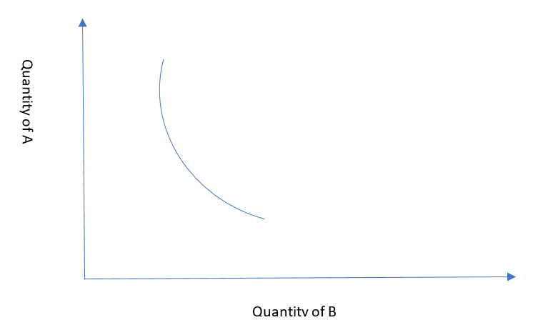
The indifference curve is a convex slope showing a relationship between two mutually exclusive inputs. It shows the optimal choice or utility at a certain point when the consumer is indifferent but equally satisfied with the choice of one input over the other.
Properties of Indifference Curve
The indifference curve holds mainly four properties. If a curve forming a relationship between two variables fulfills these properties, it will be termed an indifference curve.
- Two or more indifference curves plotted for the same variables will never cross otherwise the true utility or the optimal balance for two inputs would not be possible.
- Indifference curves plotted higher and farther to the right from the origin show a higher level of utility for the two inputs.
- An indifference curve will always have a downward slope. It means the choice of one input will come at an opportunity cost for the second and vice versa.
- The curve will have a convex shape as the marginal rate of substitution diminishes with higher consumption of the second input.
Generally, the curve will never touch the X and Y-axis on the graph as well. It simply means that this curve represents a relationship between two inputs where the consumer can choose an opportunity cost for the second one.
Understanding the Indifference Curve
Indifference covers is a simple plot on a graph representing two input variables. Each input is represented by one side of the graph X-axis or Y-Axis.
The curve of the graph shows the total utility of these two variables at any given point. This curve is drawn for inputs where the user is indifferent between choosing the right quantity of one over the second.
The curve plots the same level of total utility for both inputs though. The curve becomes a contour line with a downwards slope and a convex shape. The curve is plotted by linking each point with different variable positions for both inputs.
Suppose a buyer can purchase 50 units of two goods A and B with a total budget of $500. The consumer is indifferent between choosing the right combination as choosing over the other comes with an opportunity cost.
As the curve shows, the total utility will remain constant at 50. However, to calculate the optimal balance, we can use the following formula.
C = U (A, B)
U (A, B) represent the variable quantities of both goods A and B. C denotes the constant utility level at any given point.
If the consumer increases the budget from $500 to $1,000, the total utility increases from 50 to 100 units. It means the indifference curve shifts to the right side of the first one.
The second indifference curve will show the same downward slope and a convex shape at increased input and utility levels.
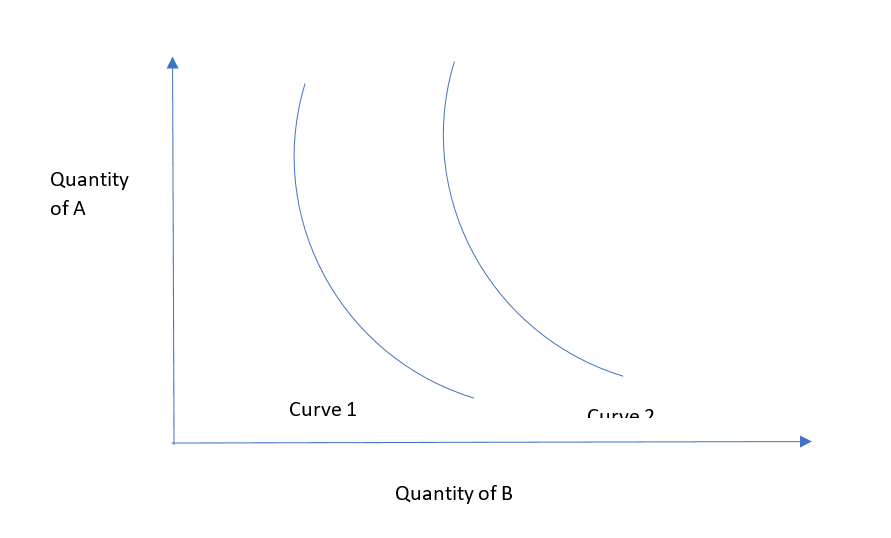
Similarly, we can draw as many indifference curves as there are varying utility levels for a set of two variables.
Indifference Curve and the Diminishing Marginal Utility Rate
The purchasing power of the consumer with a satisfaction level gained within the available resources is called utility.
In our example, the consumer could buy a total of 50 units of two goods A and B combined with a total budget of $500. The 50 units are the utility level for this consumer.
The downward slope of the curve represents the marginal rate of substitution. It means as the consumer substitutes one good with another, the slope shifts downwards.
It is the rate at which the consumer is willing to give up one good for the second one. In our example, it will be the rate at which the consumer will be willing to leave units of product A to purchase more units of product B.
However, the concept of MRS is difficult to apply in practice as many other factors like a consumer’s choice, preference, and needs determine the right combination of both products.
Optimal Utility Point on the Indifference Curve
Since there are budget constraints for a consumer, we have a defined number for the total utility. This shapes the relationship between the two inputs and results in a convex shape.
The marginal rate of substitution also means that the consumer can purchase less of product A if he wants to purchase more of product B, as in our example.
If we draw a tangent line connecting X-axis to Y-axis on the graph, the intersection point of this line of the curve will represent the optimal budget point.
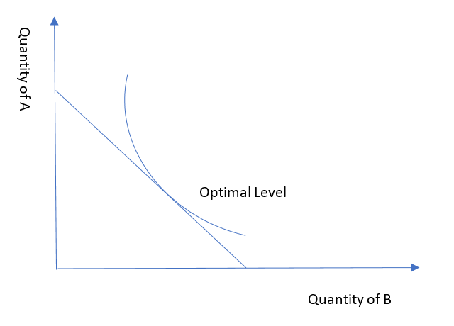
At this point, the total utility will be maximum and the number of units for both goods will be balanced.
As we can see, the budget line drops after starting higher on Y-axis to the lowest when it touches X-axis. It shows that there is always an opportunity cost.
When the consumer purchases the maximum units of product A, he will have the minimum units of product B and vice versa.
Indifference Curve Implementation
The practical use of the indifference curve depends on the right mix of inputs and some assumptions.
It is widely used to study consumer behavior in determining their preferences and spending habits. Similarly, it can be used to arrange budgets and consumer goods in the market by arranging a balanced quantity for each product.
Marketers can utilize this curve to study the impacts of different pricing strategies. For example, offering a cash discount over a quantity discount will make a consumer indifferent between two similar goods.
Economists can use this curve to study the impact of income and availability on consumer behaviors and utility rates.
As we noted above, a higher level of utility means more purchasing power for consumers. It reflects that the consumers will be willing to spend more but the total utility will remain constant.
Limitations of Indifference Curve
The indifference curve represents an economic theory that tries to rationalize consumer behavior. However, it is based on several assumptions and comes with several limitations.
First of all, consumer choices can change at any time. So, there are no rational grounds to state the consumer will always remain indifferent between two choices only.
It also means that the optimal quantity or utility does not depend on the opportunity cost but on the consumer choice and needs.
The second limitation of this theory is that it represents a relationship for two goods only. In practice, a consumer would go on to buy several products.
So, there are no solid grounds to establish a relationship between any two goods. For example, how will it shape when we plot it for an Air conditioner and an exhaust fan? The consumer will buy both of these items at different levels with different budgets.
Another limitation of the indifference curve theory is that it contradicts other theories in economics like the consumer preference theory and proportionality rule theories.